1. Quickstart — your first tracker
This is a 10-minute introduction to unitrack, the PyTorch-native multi-object tracking library. By the end of this notebook you will:
- understand what a unitrack
Trackeris (a pure step function), - build a minimal tracker that matches detections by appearance,
- run it on a synthetic clip and visualize the resulting tracks.
Subsequent tutorials drill down into each part of the library: the data model (notebook 2), the cost & gate zoos (3), the composable pipeline tree (4), state evolution and lifecycle (5), and a paper-style end-to-end reproduction (6).
What is a tracker?
A tracker associates detections (per-frame outputs of an object detector) into tracklets (per-identity sequences over time). unitrack's central abstraction is:
Tracker.step(snapshot, detections, ctx, next_id) → (snapshot', match, ids, next_id')
snapshotis the current state of the tracker — a typed, immutable record of every live tracklet's fields (id, status, age, kernel embedding, position, mask, …).detectionsis one frame's worth of new observations.ctxcarries timing and stream-identity metadata.next_idis a counter passed in by the caller for assigning new tracklet IDs.
The tracker is a pure function. It doesn't mutate its inputs;
it returns a fresh snapshot. The convenience wrapper
MultiStream holds the snapshot for you, so you don't have to
thread next_id and the snapshot through every call.
# The full set of imports we'll use across this notebook.
import torch
import matplotlib.pyplot as plt

import unitrack
from unitrack.assignment import Associate, Jonker
from unitrack.costs import Cosine
from unitrack.data import Detections, FrameContext, TensorSpec
from unitrack.lifecycle import IncludeAll, NoLifecycle
from unitrack.pipeline import Pipe
from unitrack.states import FromDetectionField, Identity, Replace, State

torch.manual_seed(0)
plt.rcParams["figure.figsize"] = (6, 4)
A minimal tracker
We'll build the simplest meaningful tracker: it matches detections across frames by cosine similarity over a learned kernel embedding.
The construction reads top-down like a recipe:
- State: each tracklet carries a
kernelfield (a 4-dim float vector).Identitymeans the predict step is a no-op (the embedding doesn't drift between frames).Replacemeans matched tracklets adopt the new detection's embedding.FromDetectionFieldsays "when a new tracklet is created, copy this field from the detection that spawned it." - Stage tree: a single
Pipethat computes a cosine-distance cost matrix and hands it toAssociate, which runs Jonker–Volgenant assignment with a 0.5 threshold. - Lifecycle / Visibility:
NoLifecycle(no Tentative→Active transitions) andIncludeAll(every tracklet is visible to the caller). The next tutorial introduces the proper lifecycle policy.
tracker = unitrack.Tracker(
    root=Pipe(cost=Cosine("kernel"), assoc=Associate(Jonker(threshold=0.5))),
    states={
        "kernel": State(
            schema=TensorSpec(shape=(4,), dtype=torch.float32),
            process=Identity("kernel"),
            observation=Replace("kernel"),
            init=FromDetectionField("kernel"),
        ),
        # `position` isn't used for matching here; we carry it on
        # the snapshot so the visualization below has a 2D point
        # to draw per tracklet.
        "position": State(
            schema=TensorSpec(shape=(2,), dtype=torch.float32),
            process=Identity("position"),
            observation=Replace("position"),
            init=FromDetectionField("position"),
        ),
    },
    lifecycle=NoLifecycle(),
    visibility=IncludeAll(),
)

ms = unitrack.MultiStream(tracker)
print(tracker)
<unitrack.tracker.tracker.Tracker object at 0x7410615a6710>
A tiny synthetic clip
We'll generate three "ground-truth" objects, each with a unique kernel embedding plus a 2D position that drifts at constant velocity. Across frames the detection order is shuffled so the tracker can't trivially exploit row alignment — it has to use the kernel embedding to reassociate.
N_FRAMES, N_OBJS, K_DIM = 8, 3, 4

# Per-identity ground truth.
kernels = torch.randn(N_OBJS, K_DIM)
kernels = kernels / kernels.norm(dim=-1, keepdim=True)
positions = torch.tensor([[20.0, 50.0], [100.0, 30.0], [180.0, 80.0]])
velocities = torch.tensor([[3.0, 1.0], [-1.0, 2.0], [-2.0, -1.0]])

clip = []
gt_per_frame = []
for k in range(N_FRAMES):
    order = torch.randperm(N_OBJS)
    gt_per_frame.append(order)

    kernel_obs = kernels[order] + 0.02 * torch.randn(N_OBJS, K_DIM)
    kernel_obs = kernel_obs / kernel_obs.norm(dim=-1, keepdim=True)
    pos_obs = positions[order] + k * velocities[order]

    clip.append(
        Detections(
            index=torch.arange(N_OBJS, dtype=torch.int64),
            kernel=kernel_obs.float(),
            position=pos_obs.float(),
            batch_size=[N_OBJS],
        )
    )
gt_per_frame = torch.stack(gt_per_frame)
print(f"Generated {N_FRAMES} frames of {N_OBJS} detections each.")
Generated 8 frames of 3 detections each.
Note Detections accepts arbitrary user fields (kernel, position)
beyond its single reserved field index. The same is true of
Tracklets. unitrack's typed-record story is intentionally
permissive about user fields so you can plug in whatever your
detector emits — kernels, masks, depth, classes, scores, …
What does the clip look like?
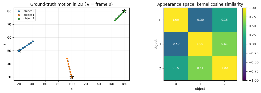
Before we track anything, let's see what we just generated — the two cues the tracker will rely on:
- Left (2D motion): each object's ground-truth position over the eight frames. This is the world the tracker observes, modulo per-frame shuffling.
- Right (appearance space): the cosine similarity between the three identities' kernel embeddings. The near-identity matrix (1 on the diagonal, ≈0 off it) is exactly what lets the cosine cost tell the objects apart even when their positions cross.
fig, (ax_pos, ax_emb) = plt.subplots(1, 2, figsize=(11, 4))
cmap = plt.get_cmap("tab10")

# (left) ground-truth motion: where each identity actually is.
for o in range(N_OBJS):
    track = torch.stack([positions[o] + k * velocities[o] for k in range(N_FRAMES)])
    ax_pos.plot(track[:, 0], track[:, 1], "-", color=cmap(o), alpha=0.4)
    ax_pos.scatter(
        track[:, 0],
        track[:, 1],
        color=cmap(o),
        s=25,
        edgecolor="black",
        linewidth=0.4,
        label=f"object {o}",
    )
    ax_pos.scatter(
        track[0, 0],
        track[0, 1],
        color=cmap(o),
        s=160,
        marker="*",
        edgecolor="black",
        zorder=3,
    )
ax_pos.set_title("Ground-truth motion in 2D (★ = frame 0)")
ax_pos.set_xlabel("x")
ax_pos.set_ylabel("y")
ax_pos.legend(fontsize=8)
ax_pos.grid(alpha=0.3)

# (right) appearance space: cosine similarity between identity kernels.
sim = kernels @ kernels.T
im = ax_emb.imshow(sim.numpy(), cmap="viridis", vmin=-1, vmax=1)
ax_emb.set_title("Appearance space: kernel cosine similarity")
ax_emb.set_xlabel("object")
ax_emb.set_ylabel("object")
ax_emb.set_xticks(range(N_OBJS))
ax_emb.set_yticks(range(N_OBJS))
for i in range(N_OBJS):
    for j in range(N_OBJS):
        ax_emb.text(
            j,
            i,
            f"{sim[i, j]:.2f}",
            ha="center",
            va="center",
            color="white",
            fontsize=9,
        )
fig.colorbar(im, ax=ax_emb, fraction=0.046)
plt.tight_layout()
plt.show()
Run the tracker
Each step takes one frame's detections and a FrameContext (which
carries the frame index and a delta-t for state evolution). The
wrapper holds the snapshot internally and threads next_id through.
all_results = []
for k, dets in enumerate(clip):
    ctx = FrameContext.make(frame_idx=k, delta=1 / 15.0, fps=15.0, stream_key=0)
    res = ms.step(stream_key=0, detections=dets, ctx=ctx)
    all_results.append(res)
    print(
        f"frame {k}: snapshot={res.snapshot.batch_size[0]} live, ids={res.ids.tolist()}"
    )
frame 0: snapshot=3 live, ids=[1, 2, 3]
frame 1: snapshot=3 live, ids=[1, 2, 3]
frame 2: snapshot=3 live, ids=[1, 2, 3]
frame 3: snapshot=3 live, ids=[1, 2, 3]
frame 4: snapshot=3 live, ids=[1, 2, 3]
frame 5: snapshot=3 live, ids=[1, 2, 3]
frame 6: snapshot=3 live, ids=[1, 2, 3]
frame 7: snapshot=3 live, ids=[1, 2, 3]
Three tracklets live across all eight frames. Their IDs (1, 2, 3) are stable — the tracker correctly matches every shuffled detection back to the right identity by cosine similarity on the kernel.
Visualize
We'll draw the trajectories color-coded by tracker-assigned ID. Each marker is one detection, located at its 2D position; the color tells us which tracklet the tracker thinks it belongs to.
fig, ax = plt.subplots(figsize=(8, 5))
cmap = plt.get_cmap("tab10")

for k, (dets, res) in enumerate(zip(clip, all_results)):
    # The snapshot's id field aligns with the matched-then-appended order.
    # For this minimal example we re-derive per-detection IDs by walking
    # the snapshot in detection-index order. (Notebook 6 shows a robust
    # version of this for ground-truth evaluation.)
    ids = res.snapshot.id
    pos = res.snapshot.position
    for n, tid in enumerate(ids):
        ax.scatter(
            pos[n, 0],
            pos[n, 1],
            color=cmap(int(tid) % 10),
            s=40,
            edgecolor="black",
            linewidth=0.5,
        )
        if k == 0:
            ax.text(pos[n, 0] + 5, pos[n, 1], f"id={int(tid)}", fontsize=9)

ax.set_xlabel("x")
ax.set_ylabel("y")
ax.set_title("Per-detection track IDs over 8 frames (color = tracker ID)")
ax.grid(alpha=0.3)
plt.show()
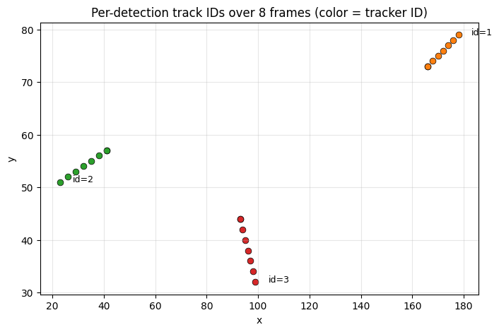
Each color forms a coherent trajectory in (x, y) — the tracker preserved identity across all 8 frames, despite per-frame detection shuffling.
What's next
- Notebook 2 unpacks the typed records (
Tracklets,Detections,CostExpression,MatchOutcome,Gate) and explains why unitrack uses immutable snapshots. - Notebook 3 visualizes every cost and gate primitive in the library.
- Notebook 4 builds richer pipelines with
Sequential,Parallel,Gated,Filter, andIterate. - Notebook 5 introduces state evolution (Kalman, EMA) and lifecycle (Tentative → Active → Lost → Removed).
- Notebook 6 assembles a K=2 cascaded canonical configuration and compares cascaded vs parallel fusion end-to-end.