Notebook

Kalman filters for motion prediction in tracking

A tracker has to answer one question every frame: given everything I have seen so far, where is each object now — and how sure am I? A Kalman filter answers both at once. It carries, per object, a Gaussian belief over a latent state (position, velocity, size, …) and rolls it forward in two steps:

Predict — push the belief through a motion model $x' = F x$ , and grow its covariance $P' = F P F^\top + Q$ . This is the filter's guess about the next frame, before it sees any detection. It is a full distribution, not a point.
Update — when a detection arrives, fuse it (Joseph-form Kalman gain), pulling the mean toward the measurement and shrinking the covariance by however much the measurement was worth.

This notebook visualizes that loop for the five state types unitrack ships a Kalman model for:

State	unitrack class	latent state	measurement
2-D point	`KalmanCentroid2D`	`[x, y, vx, vy]`	`[x, y]`
2-D box	`KalmanBBox` (SORT)	`[x, y, a, h, vx, vy, va]`	`[x, y, a, h]`
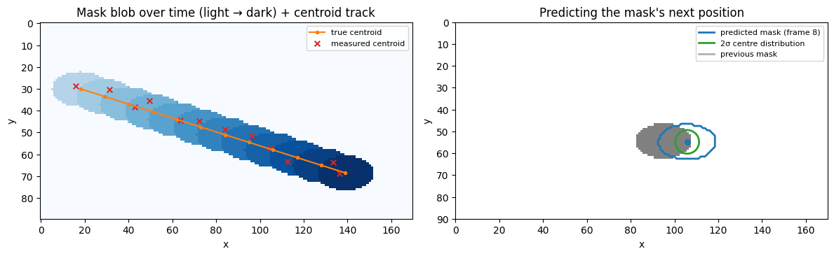
2-D mask	`KalmanCentroid2D` on the mask centroid	`[x, y, vx, vy]`	`[x, y]`
3-D point cloud	`KalmanCentroid3D`	`[x,y,z, vx,vy,vz]`	`[x, y, z]`
kernel / appearance	`KalmanLinear` (random walk)	`[e₁ … e_d]`	`[e₁ … e_d]`

For points, boxes and masks we draw the object's trajectory over time and the filter's one-step-ahead predictive distribution — the ellipse it would hand an association gate as "the detection should land about here." The last section stress-tests the filter: where it shines (occlusion, noise) and where it breaks (maneuvers, bad tuning, crossing targets).

Setup

Everything here is pure unitrack + matplotlib. We drive the Kalman Process (predict) and its paired KalmanUpdate (observation) directly, frame by frame, instead of wrapping them in a full Tracker — that keeps the belief itself in view, which is the whole point.

import math

import numpy as np
import torch
import matplotlib.pyplot as plt
from matplotlib.patches import Ellipse, Rectangle

from unitrack.data import Detections, FrameContext, MatchOutcome, Tracklets
from unitrack.lifecycle import TrackletStatus
from unitrack.states.kalman import (
    KalmanBBox, KalmanCentroid2D, KalmanCentroid3D,
    KalmanLinear, KalmanUpdate,
)

torch.manual_seed(0)
plt.rcParams["figure.figsize"] = (7, 4)

A thin driver around the unitrack Kalman API

KalmanCentroid2D, KalmanCentroid3D and KalmanBBox are each a Process (the predict step, proc(cs, ctx)) plus a make_update() factory that returns the matching KalmanUpdate. Both read the mean from cs.{field} and the covariance from cs.{field}_cov. The helpers below wrap a single object into a one-row Tracklets snapshot and run a sequence of measurements through predict → (optional) update, recording the belief at every frame.

def one_tracklet(field, mean, cov):
    """Wrap a single (mean, cov) pair into a 1-row Tracklets snapshot."""
    return Tracklets(
        id=torch.tensor([1], dtype=torch.int64),
        status=torch.tensor([int(TrackletStatus.Active)], dtype=torch.int8),
        hits=torch.tensor([1], dtype=torch.int32),
        time_since_update=torch.zeros(1, dtype=torch.int32),
        age=torch.ones(1, dtype=torch.int32),
        frame_started=torch.zeros(1, dtype=torch.int32),
        frame_last_seen=torch.zeros(1, dtype=torch.int32),
        **{field: mean.unsqueeze(0).float(),
           f"{field}_cov": cov.unsqueeze(0).float()},
        batch_size=[1],
    )

def match_one():
    """A MatchOutcome pairing tracklet 0 with detection 0."""
    return MatchOutcome(
        matched_pairs=torch.tensor([[0, 0]], dtype=torch.int64),
        tracklets_residual_index=torch.zeros(0, dtype=torch.int64),
        detections_residual_index=torch.zeros(0, dtype=torch.int64),
        per_match_cost=torch.zeros(1),
        batch_size=[],
    )

def run_kalman(proc, init_mean, init_cov, measurements, present, *,
               dt=1.0, dts=None, gate_chi2=None):
    """
    Drive a unitrack Kalman process over a sequence.

    Returns one record per frame holding the *prior* (post-predict,
    pre-update) belief — where the filter expects the object to be
    *before* the new detection — and the *posterior* after fusion.
    On a missed frame (``present[k]`` False) no update runs, so the
    prior carries forward: pure coasting.

    Parameters
    ----------
    dt : float
        Constant time step (used when ``dts`` is None).
    dts : sequence of float, optional
        Per-frame time step, for irregular frame rates. Each predict
        uses ``delta=dts[k]`` so ``F`` and ``Q`` scale with real time.
    gate_chi2 : float, optional
        If set, a detection whose squared Mahalanobis distance to the
        predictive distribution exceeds this threshold is *rejected*
        (treated as a miss). This is the standard outlier gate; the
        record's ``"gated"`` flag marks rejected frames.
    """
    field = proc.field
    upd = proc.make_update()
    snap = one_tracklet(field, init_mean, init_cov)
    out = []
    for k, seen in enumerate(present):
        delta = float(dts[k]) if dts is not None else dt
        ctx = FrameContext.make(frame_idx=k, delta=delta)
        snap = proc(snap, ctx)                              # PREDICT
        prior_mean = getattr(snap, field)[0].clone()
        prior_cov = getattr(snap, f"{field}_cov")[0].clone()
        rec = {"prior_mean": prior_mean, "prior_cov": prior_cov,
               "seen": seen, "gated": False}
        if seen:
            z = measurements[k].float()
            m = z.shape[0]
            if gate_chi2 is not None:
                S = prior_cov[:m, :m] + torch.eye(m) * proc.r
                inn = (z - prior_mean[:m]).double()
                md2 = float(inn @ torch.linalg.inv(S.double()) @ inn)
                rec["gated"] = md2 > gate_chi2
            if not rec["gated"]:
                ds = Detections(index=torch.tensor([0], dtype=torch.int64),
                                **{field: z.unsqueeze(0)}, batch_size=[1])
                snap = upd(snap, ds, match_one(), ctx)     # UPDATE
        rec["post_mean"] = getattr(snap, field)[0].clone()
        rec["post_cov"] = getattr(snap, f"{field}_cov")[0].clone()
        out.append(rec)
    return out

# --- plotting helpers -------------------------------------------------

def cov_ellipse(ax, mean2, cov2, n_std=2.0, **kw):
    """Draw an n-sigma covariance ellipse for a 2-D Gaussian."""
    cov2 = cov2.detach().cpu().double()
    vals, vecs = torch.linalg.eigh(cov2)
    vals = vals.clamp(min=1e-12)
    order = torch.argsort(vals, descending=True)
    vals, vecs = vals[order], vecs[:, order]
    angle = math.degrees(math.atan2(float(vecs[1, 0]), float(vecs[0, 0])))
    width, height = (2 * n_std * vals.sqrt()).tolist()
    ax.add_patch(Ellipse((float(mean2[0]), float(mean2[1])),
                         width, height, angle=angle, fill=False, **kw))

def predictive_xy(rec, r, n=2):
    """
    One-step-ahead measurement distribution for the position block.

    For these models H = [I | 0], so the predicted measurement mean
    is the leading ``n`` state entries and its covariance is the
    leading n-by-n block of P plus the measurement noise R = r*I.
    """
    mu = rec["prior_mean"][:n]
    S = rec["prior_cov"][:n, :n] + torch.eye(n) * r
    return mu, S

def fade(cmap_name, k, n):
    """A time-graded color: early frames light, late frames saturated."""
    return plt.get_cmap(cmap_name)(0.25 + 0.7 * k / max(1, n - 1))

1 — Points: a 2-D centroid

The canonical case. A constant-velocity object drifts across the frame; the detector reports its centroid with Gaussian noise. KalmanCentroid2D carries [x, y, vx, vy] and observes [x, y].

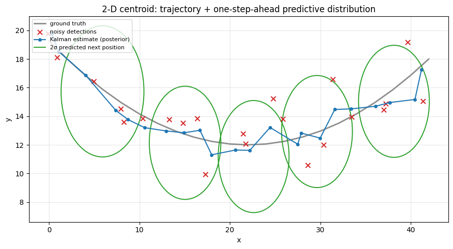
Below, the grey curve is the true path, red ✕ are the noisy detections, and the blue line is the filter's posterior estimate. The green ellipses are what makes the filter a filter: at sampled frames, the 2σ region where the filter — using only past detections — expects the next detection to fall. A χ²/Mahalanobis gate is exactly "is the detection inside this ellipse?".

T = 22
t = torch.arange(T).float()
true_xy = torch.stack([2.0 * t, 12.0 + 0.06 * (t - 11) ** 2], dim=1)
g = torch.Generator().manual_seed(3)
sigma = 1.4
meas = true_xy + sigma * torch.randn(T, 2, generator=g)

proc = KalmanCentroid2D("centroid", q=0.08, r=sigma ** 2)
init_mean = torch.tensor([float(meas[0, 0]), float(meas[0, 1]), 2.0, 0.0])
init_cov = torch.diag(torch.tensor([4.0, 4.0, 4.0, 4.0]))
rec = run_kalman(proc, init_mean, init_cov, list(meas), [True] * T)
post = torch.stack([r["post_mean"][:2] for r in rec])

fig, ax = plt.subplots(figsize=(9, 5))
ax.plot(true_xy[:, 0], true_xy[:, 1], "-", color="0.55", lw=2,
        label="ground truth", zorder=1)
ax.scatter(meas[:, 0], meas[:, 1], marker="x", color="tab:red", s=45,
           label="noisy detections", zorder=2)
ax.plot(post[:, 0], post[:, 1], "o-", color="tab:blue", ms=4,
        label="Kalman estimate (posterior)", zorder=3)
for k in range(3, T, 4):
    mu, S = predictive_xy(rec[k], proc.r)
    cov_ellipse(ax, mu, S, n_std=2.0, edgecolor="tab:green", lw=1.4)
ax.plot([], [], color="tab:green", lw=1.4,
        label="2σ predicted next position")
ax.set_title("2-D centroid: trajectory + one-step-ahead predictive distribution")
ax.set_xlabel("x"); ax.set_ylabel("y")
ax.legend(loc="upper left", fontsize=8); ax.grid(alpha=0.3)
plt.tight_layout(); plt.show()

Predicting through an occlusion

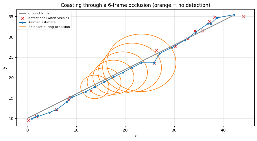
The predictive distribution is most useful when there is no detection to fall back on. Here the object is occluded for six frames (no detections, frames 7–12). With no measurement to fuse, the filter keeps predicting: the mean coasts along the last known velocity and the covariance grows every frame — the ellipses balloon, honestly reporting "it's somewhere in here, and I'm less and less sure." When the object reappears, one detection collapses the uncertainty again.

present = [True] * 7 + [False] * 6 + [True] * 9
T2 = len(present)
t2 = torch.arange(T2).float()
true2 = torch.stack([2.0 * t2, 10.0 + 1.2 * t2], dim=1)
g = torch.Generator().manual_seed(5)
meas2 = true2 + 1.0 * torch.randn(T2, 2, generator=g)

proc = KalmanCentroid2D("centroid", q=0.05, r=1.0)
init_mean = torch.tensor([float(meas2[0, 0]), float(meas2[0, 1]), 2.0, 1.2])
rec2 = run_kalman(proc, init_mean, torch.eye(4) * 3.0,
                  list(meas2), present)
est2 = torch.stack([r["post_mean"][:2] for r in rec2])

fig, ax = plt.subplots(figsize=(9, 5))
ax.plot(true2[:, 0], true2[:, 1], "-", color="0.55", lw=2, label="ground truth")
seen_mask = torch.tensor(present)
ax.scatter(meas2[seen_mask, 0], meas2[seen_mask, 1], marker="x",
           color="tab:red", s=45, label="detections (when visible)")
ax.plot(est2[:, 0], est2[:, 1], "o-", color="tab:blue", ms=4,
        label="Kalman estimate")
for k in range(T2):
    if not present[k]:                      # draw the growing belief
        mu, S = predictive_xy(rec2[k], proc.r)
        cov_ellipse(ax, mu, S, n_std=2.0, edgecolor="tab:orange", lw=1.3)
ax.plot([], [], color="tab:orange", lw=1.3, label="2σ belief during occlusion")
ax.set_title("Coasting through a 6-frame occlusion (orange = no detection)")
ax.set_xlabel("x"); ax.set_ylabel("y")
ax.legend(loc="upper left", fontsize=8); ax.grid(alpha=0.3)
plt.tight_layout(); plt.show()

2 — 2-D boxes

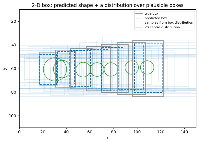
KalmanBBox (the SORT model) tracks a box as [x, y, a, h] — centre, aspect ratio a = w/h, and height h — with velocities on centre and aspect. That means the filter predicts not just where the box goes but how it reshapes. Here a box translates right and grows taller; the detector reports noisy [x, y, a, h].

We draw the true box (grey) and the predicted box (blue) at sampled frames. The green ellipse is the predictive distribution of the box centre; the faint blue boxes are samples drawn from the full predictive [x, y, a, h] distribution — a "cloud of plausible boxes" the filter is offering for the next frame.

T = 14
t = torch.arange(T).float()
cx, cy = 25.0 + 7.0 * t, 60.0 + torch.zeros(T)
h = 28.0 + 1.6 * t                       # growing height
a = torch.full((T,), 0.55)               # aspect ratio w/h
true_box = torch.stack([cx, cy, a, h], dim=1)        # [x, y, a, h]
g = torch.Generator().manual_seed(7)
noise = torch.tensor([2.0, 2.0, 0.03, 2.0])
meas_box = true_box + noise * torch.randn(T, 4, generator=g)

proc = KalmanBBox("bbox", q=0.2, r=4.0, model="sort")   # 7-D SORT state
init_mean = torch.zeros(7)
init_mean[:4] = meas_box[0]
init_mean[4] = 7.0                                      # vx prior
rec_box = run_kalman(proc, init_mean, torch.eye(7) * 10.0,
                     list(meas_box), [True] * T)

def draw_box(ax, xyah, **kw):
    x, y, asp, hh = [float(v) for v in xyah[:4]]
    w = asp * hh
    ax.add_patch(Rectangle((x - w / 2, y - hh / 2), w, hh, fill=False, **kw))

fig, ax = plt.subplots(figsize=(9, 5))
for k in range(0, T, 2):
    draw_box(ax, true_box[k], edgecolor="0.6", lw=2)
    draw_box(ax, rec_box[k]["post_mean"], edgecolor="tab:blue", lw=1.5,
             linestyle="--")
    # samples from the predictive [x, y, a, h] distribution
    mu4 = rec_box[k]["prior_mean"][:4]
    S4 = rec_box[k]["prior_cov"][:4, :4] + torch.eye(4) * proc.r
    S4 = S4 + torch.eye(4) * 1e-6
    dist = torch.distributions.MultivariateNormal(mu4.double(), S4.double())
    for _ in range(12):
        draw_box(ax, dist.sample().float(), edgecolor="tab:blue",
                 lw=0.5, alpha=0.18)
    mu, S = predictive_xy(rec_box[k], proc.r)
    cov_ellipse(ax, mu, S, n_std=2.0, edgecolor="tab:green", lw=1.2)
ax.plot([], [], color="0.6", lw=2, label="true box")
ax.plot([], [], color="tab:blue", lw=1.5, ls="--", label="predicted box")
ax.plot([], [], color="tab:blue", lw=0.5, label="samples from box distribution")
ax.plot([], [], color="tab:green", lw=1.2, label="2σ centre distribution")
ax.set_xlim(0, 150); ax.set_ylim(110, 10)            # image convention
ax.set_aspect("equal")
ax.set_title("2-D box: predicted shape + a distribution over plausible boxes")
ax.set_xlabel("x"); ax.set_ylabel("y"); ax.legend(fontsize=8)
plt.tight_layout(); plt.show()

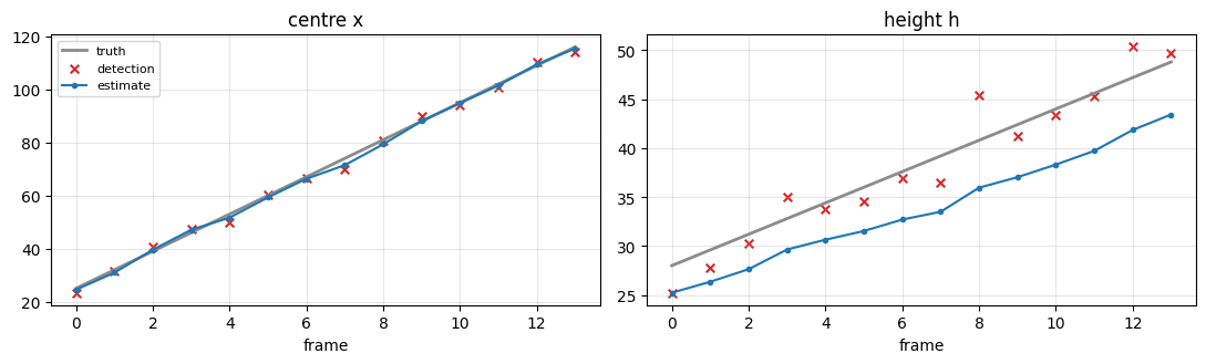
# The same run, as time series: the filter predicts size as well as place.
post_box = torch.stack([r["post_mean"] for r in rec_box])
fig, axes = plt.subplots(1, 2, figsize=(11, 3.4))
for ax, j, name in [(axes[0], 0, "centre x"), (axes[1], 3, "height h")]:
    ax.plot(t, true_box[:, j], "-", color="0.55", lw=2, label="truth")
    ax.scatter(t, meas_box[:, j], marker="x", color="tab:red", s=30,
               label="detection")
    ax.plot(t, post_box[:, j], "o-", color="tab:blue", ms=3, label="estimate")
    ax.set_title(name); ax.set_xlabel("frame"); ax.grid(alpha=0.3)
axes[0].legend(fontsize=8)
plt.tight_layout(); plt.show()

3 — 2-D masks

A segmentation mask is a bitmap, not a vector — a Kalman filter cannot smooth pixels directly. The standard move is to track a low-dimensional summary of the mask (here its centroid) with KalmanCentroid2D, and carry the mask shape along for rendering. The prediction then says "the blob's centre will be about here, with this uncertainty," and you translate the mask template to that centre.

Left: the mask at each frame, time-graded light→dark, with the true centroid path. Right: at one frame, the predicted mask (translated to the prior centroid) and the 2σ ellipse for where the centre will land.

Himg, Wimg = 90, 170
ys, xs = torch.meshgrid(torch.arange(Himg), torch.arange(Wimg), indexing="ij")

def make_mask(cx, cy, rx=13.0, ry=8.0):
    return (((xs - cx) / rx) ** 2 + ((ys - cy) / ry) ** 2) <= 1.0

def mask_centroid(mask):
    idx = mask.nonzero().float()                     # rows are [y, x]
    return torch.stack([idx[:, 1].mean(), idx[:, 0].mean()])   # [x, y]

T = 12
t = torch.arange(T).float()
true_c = torch.stack([18.0 + 11.0 * t, 30.0 + 3.5 * t], dim=1)
masks = [make_mask(float(cx), float(cy)) for cx, cy in true_c]
g = torch.Generator().manual_seed(9)
meas_c = torch.stack([mask_centroid(m) for m in masks])             + 2.0 * torch.randn(T, 2, generator=g)

proc = KalmanCentroid2D("centroid", q=0.1, r=4.0)
init_mean = torch.tensor([float(meas_c[0, 0]), float(meas_c[0, 1]), 11.0, 3.5])
rec_m = run_kalman(proc, init_mean, torch.eye(4) * 6.0,
                   list(meas_c), [True] * T)

fig, (axL, axR) = plt.subplots(1, 2, figsize=(12, 4))

# (left) masks over time + centroid trajectory
composite = torch.zeros(Himg, Wimg)
for k, m in enumerate(masks):
    composite = torch.maximum(composite, m.float() * (0.3 + 0.7 * k / (T - 1)))
axL.imshow(composite.numpy(), cmap="Blues", origin="upper")
axL.plot(true_c[:, 0], true_c[:, 1], "-o", color="tab:orange", ms=3,
         label="true centroid")
axL.scatter(meas_c[:, 0], meas_c[:, 1], marker="x", color="tab:red", s=30,
            label="measured centroid")
axL.set_title("Mask blob over time (light → dark) + centroid track")
axL.legend(fontsize=8); axL.set_xlabel("x"); axL.set_ylabel("y")

# (right) predicted mask + centre uncertainty at frame kf
kf = 8
axR.imshow(masks[kf - 1].numpy(), cmap="Greys", origin="upper", alpha=0.5)
pri = rec_m[kf]["prior_mean"][:2]
template = make_mask(float(pri[0]), float(pri[1]))   # mask at predicted centre
axR.contour(template.numpy(), levels=[0.5], colors="tab:blue", linewidths=2)
mu, S = predictive_xy(rec_m[kf], proc.r)
cov_ellipse(axR, mu, S, n_std=2.0, edgecolor="tab:green", lw=2)
axR.scatter([float(pri[0])], [float(pri[1])], color="tab:blue", s=30, zorder=3)
axR.plot([], [], color="tab:blue", lw=2, label="predicted mask (frame %d)" % kf)
axR.plot([], [], color="tab:green", lw=2, label="2σ centre distribution")
axR.plot([], [], color="0.4", lw=2, alpha=0.5, label="previous mask")
axR.set_xlim(0, Wimg); axR.set_ylim(Himg, 0)
axR.set_title("Predicting the mask's next position")
axR.legend(fontsize=8); axR.set_xlabel("x"); axR.set_ylabel("y")
plt.tight_layout(); plt.show()

4 — 3-D point clouds

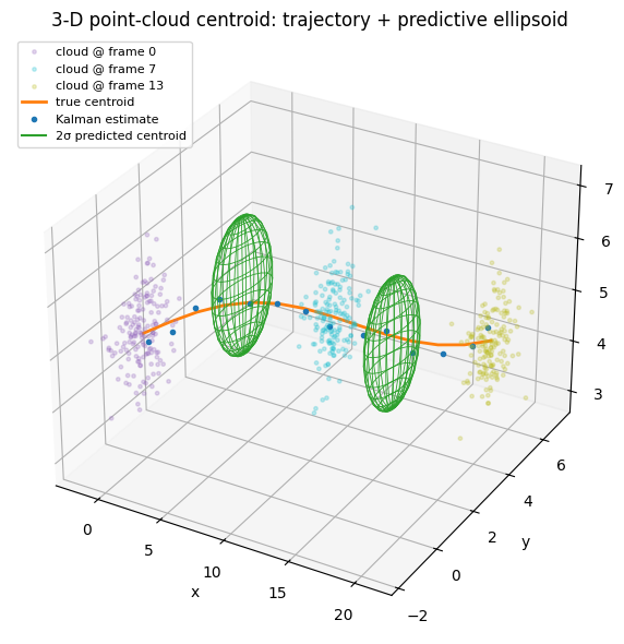
For LiDAR-style tracking the object is a cloud of 3-D points; its location is summarized by the cloud centroid, tracked with KalmanCentroid3D (state [x,y,z, vx,vy,vz], measurement [x, y, z]). The predictive distribution is now a 3-D Gaussian — we draw it as a 2σ wireframe ellipsoid around the predicted centroid.

The faded clouds show the object at three frames; the orange line is the true centroid path; the green ellipsoid is where the filter expects the centroid next, given only the earlier frames.

def plot_ellipsoid(ax, mean3, cov3, n_std=2.0, **kw):
    cov3 = cov3.detach().cpu().double().numpy()
    u = np.linspace(0, 2 * np.pi, 24)
    v = np.linspace(0, np.pi, 14)
    sphere = np.stack([
        np.outer(np.cos(u), np.sin(v)),
        np.outer(np.sin(u), np.sin(v)),
        np.outer(np.ones_like(u), np.cos(v)),
    ]).reshape(3, -1)
    L = np.linalg.cholesky(cov3 + np.eye(3) * 1e-9) * n_std
    pts = (L @ sphere) + mean3.detach().cpu().numpy()[:, None]
    P = pts.reshape(3, u.size, v.size)
    ax.plot_wireframe(P[0], P[1], P[2], **kw)

T = 14
t = torch.arange(T).float()
true_c3 = torch.stack([1.5 * t, 0.4 * t, 5.0 + 0.5 * torch.sin(0.4 * t)], dim=1)
g = torch.Generator().manual_seed(11)
clouds = [c + 0.6 * torch.randn(160, 3, generator=g) for c in true_c3]
meas_c3 = torch.stack([cloud.mean(0) for cloud in clouds])             + 0.25 * torch.randn(T, 3, generator=g)

proc = KalmanCentroid3D("centroid", q=0.05, r=0.1)
init_mean = torch.zeros(6)
init_mean[:3] = meas_c3[0]
init_mean[3:5] = torch.tensor([1.5, 0.4])
rec3 = run_kalman(proc, init_mean, torch.eye(6) * 2.0,
                  list(meas_c3), [True] * T)
post3 = torch.stack([r["post_mean"][:3] for r in rec3])

fig = plt.figure(figsize=(9, 6))
ax = fig.add_subplot(projection="3d")
for k, col in [(0, "tab:purple"), (T // 2, "tab:cyan"), (T - 1, "tab:olive")]:
    c = clouds[k]
    ax.scatter(c[:, 0], c[:, 1], c[:, 2], s=6, alpha=0.25, color=col,
               label=f"cloud @ frame {k}")
ax.plot(true_c3[:, 0], true_c3[:, 1], true_c3[:, 2], "-", color="tab:orange",
        lw=2, label="true centroid")
ax.plot(post3[:, 0], post3[:, 1], post3[:, 2], "o", color="tab:blue", ms=3,
        label="Kalman estimate")
for k in (4, 9):
    mu3 = rec3[k]["prior_mean"][:3]
    S3 = rec3[k]["prior_cov"][:3, :3] + torch.eye(3) * proc.r
    plot_ellipsoid(ax, mu3, S3, n_std=2.0, color="tab:green", lw=0.6)
ax.plot([], [], color="tab:green", label="2σ predicted centroid")
ax.set_xlabel("x"); ax.set_ylabel("y"); ax.set_zlabel("z")
ax.set_title("3-D point-cloud centroid: trajectory + predictive ellipsoid")
ax.legend(fontsize=8, loc="upper left")
plt.tight_layout(); plt.show()

5 — Kernel / appearance states

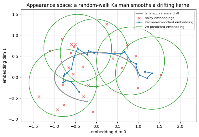
Appearance embeddings (ReID kernels) have no velocity — there is no "motion model" for a feature vector. But a Kalman filter still helps: model the embedding as a random walk (F = I, so the predict step only inflates covariance) and the update becomes a principled, uncertainty-weighted smoother — EMA's grown-up cousin, where the blend rate is set by how trustworthy each observation is rather than a fixed ρ.

We build this directly from the KalmanLinear backbone with F = H = I. The embedding is 2-D here so we can watch it; in practice it is 512-D, but the recursion is identical. A slowly drifting appearance (lighting, pose) is tracked through heavy per-frame noise.

class RandomWalkKalman:
    """F = H = I Kalman: a smoother for no-motion (appearance) states."""
    def __init__(self, field, dim, q, r):
        self.field, self.dim, self.r = field, dim, r
        eye = torch.eye(dim)
        self._proc = KalmanLinear(field=field, F=eye, H=eye,
                                  Q=eye * q, R=eye * r)
        self._upd = KalmanUpdate(field=field, cov_field=f"{field}_cov",
                                 H=eye, R=eye * r)
    def __call__(self, cs, ctx):
        return self._proc(cs, ctx)
    def make_update(self):
        return self._upd

T = 26
t = torch.arange(T).float()
true_emb = torch.stack([torch.cos(0.18 * t), 0.6 * torch.sin(0.18 * t)], dim=1)
g = torch.Generator().manual_seed(13)
emb_noise = 0.35
meas_emb = true_emb + emb_noise * torch.randn(T, 2, generator=g)

proc = RandomWalkKalman("emb", dim=2, q=0.01, r=emb_noise ** 2)
rec_e = run_kalman(proc, meas_emb[0], torch.eye(2) * 0.3,
                   list(meas_emb), [True] * T)
post_e = torch.stack([r["post_mean"] for r in rec_e])

fig, ax = plt.subplots(figsize=(7, 6))
ax.plot(true_emb[:, 0], true_emb[:, 1], "-", color="0.55", lw=2,
        label="true appearance drift")
ax.scatter(meas_emb[:, 0], meas_emb[:, 1], marker="x", color="tab:red",
           s=35, alpha=0.7, label="noisy embeddings")
ax.plot(post_e[:, 0], post_e[:, 1], "o-", color="tab:blue", ms=3,
        label="Kalman-smoothed embedding")
for k in range(2, T, 5):
    mu, S = predictive_xy(rec_e[k], proc.r)
    cov_ellipse(ax, mu, S, n_std=2.0, edgecolor="tab:green", lw=1.2)
ax.plot([], [], color="tab:green", lw=1.2, label="2σ predicted embedding")
ax.set_title("Appearance space: a random-walk Kalman smooths a drifting kernel")
ax.set_xlabel("embedding dim 0"); ax.set_ylabel("embedding dim 1")
ax.legend(fontsize=8); ax.set_aspect("equal"); ax.grid(alpha=0.3)
plt.tight_layout(); plt.show()

A caveat worth stating: a linear-Gaussian filter lives in flat Euclidean space, but ReID embeddings usually live on the unit sphere (cosine similarity). Smoothing then nudging back onto the sphere (re-normalising) is a pragmatic hack, not exact inference — which is why appearance is the state type where Kalman is least natural, and a fixed-rate EMA is often preferred. Use it when the embedding really does wander slowly and you want uncertainty-aware blending.

6 — Complex examples: where it works, where it breaks

The Kalman filter is optimal only when its assumptions hold: a linear motion model, Gaussian noise, and noise covariances Q (process) and R (measurement) that actually match reality. Tracking violates all three routinely. This section makes the failure modes concrete — each is a situation you will meet in a real video.

6a — Success: heavy noise, steady motion

The case the filter was made for. Measurement noise is large, but the motion is genuinely constant-velocity, so averaging over time wins: the estimate is far smoother and closer to truth than the raw detections. This is the baseline "it just works."

T = 30
t = torch.arange(T).float()
truth = torch.stack([1.5 * t, 0.8 * t], dim=1)
g = torch.Generator().manual_seed(21)
noisy = truth + 3.0 * torch.randn(T, 2, generator=g)
proc = KalmanCentroid2D("centroid", q=0.02, r=9.0)
m0 = torch.tensor([float(noisy[0, 0]), float(noisy[0, 1]), 1.5, 0.8])
rec = run_kalman(proc, m0, torch.eye(4) * 5.0, list(noisy), [True] * T)
est = torch.stack([r["post_mean"][:2] for r in rec])
rms_raw = (noisy - truth).pow(2).sum(1).mean().sqrt()
rms_kf = (est - truth).pow(2).sum(1).mean().sqrt()

fig, ax = plt.subplots(figsize=(8, 4))
ax.plot(truth[:, 0], truth[:, 1], "-", color="0.55", lw=2, label="truth")
ax.scatter(noisy[:, 0], noisy[:, 1], marker="x", color="tab:red", s=30,
           alpha=0.6, label=f"detections (RMS {rms_raw:.2f})")
ax.plot(est[:, 0], est[:, 1], "o-", color="tab:blue", ms=3,
        label=f"Kalman (RMS {rms_kf:.2f})")
ax.set_title("Success: the filter denoises a constant-velocity track")
ax.legend(fontsize=8); ax.grid(alpha=0.3)
plt.tight_layout(); plt.show()
print(f"raw detection RMS error: {rms_raw:.2f}   Kalman RMS error: {rms_kf:.2f}")

Output

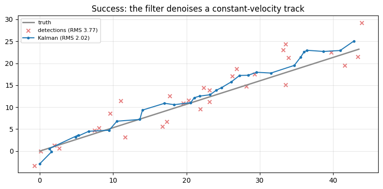
raw detection RMS error: 3.77   Kalman RMS error: 2.02

6b — Failure: a maneuvering target

A constant-velocity model assumes the object does not accelerate. When the target makes a hard 90° turn, the filter — still confident in the old velocity — overshoots, and for several frames the true position falls outside the 2σ predictive ellipse. In a real tracker that is fatal: a Mahalanobis gate would reject the correct detection as too far away, and the track either dies or steals someone else's detection. The red ✕ marks frames where the truth is outside the gate.

# An L-shaped path: east for 10 frames, then a sharp turn north.
leg = torch.arange(10).float()
east = torch.stack([3.0 * leg, torch.zeros(10)], dim=1)
north = torch.stack([27.0 + torch.zeros(12), 3.0 * torch.arange(1, 13).float()],
                    dim=1)
truth = torch.cat([east, north], dim=0)
T = truth.shape[0]
g = torch.Generator().manual_seed(23)
meas = truth + 0.6 * torch.randn(T, 2, generator=g)

proc = KalmanCentroid2D("centroid", q=0.05, r=0.4)
m0 = torch.tensor([0.0, 0.0, 3.0, 0.0])
rec = run_kalman(proc, m0, torch.eye(4) * 2.0, list(meas), [True] * T)
est = torch.stack([r["post_mean"][:2] for r in rec])

# Which frames is the truth outside the 2-sigma predictive gate?
outside = []
for k in range(T):
    mu, S = predictive_xy(rec[k], proc.r)
    d = (truth[k] - mu).double()
    md2 = float(d @ torch.linalg.inv(S.double()) @ d)   # squared Mahalanobis
    outside.append(md2 > 5.991)                          # chi2(2dof, .95)

fig, ax = plt.subplots(figsize=(8, 5))
ax.plot(truth[:, 0], truth[:, 1], "-", color="0.55", lw=2, label="truth (turns!)")
ax.plot(est[:, 0], est[:, 1], "o-", color="tab:blue", ms=3, label="Kalman estimate")
for k in range(8, T):
    mu, S = predictive_xy(rec[k], proc.r)
    col = "tab:red" if outside[k] else "tab:green"
    cov_ellipse(ax, mu, S, n_std=2.0, edgecolor=col, lw=1.1, alpha=0.7)
miss = torch.tensor(outside)
ax.scatter(truth[miss, 0], truth[miss, 1], marker="x", color="tab:red", s=70,
           zorder=4, label="truth outside 2σ gate")
ax.plot([], [], color="tab:green", label="gate covers truth")
ax.set_title("Failure: CV model lags a maneuver; the gate rejects the truth")
ax.legend(fontsize=8); ax.grid(alpha=0.3); ax.set_aspect("equal")
plt.tight_layout(); plt.show()
print(f"frames where truth left the 2σ gate: {int(miss.sum())} / {T}")

Output

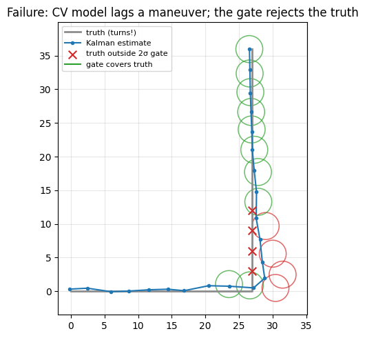
frames where truth left the 2σ gate: 4 / 22

The fix in practice is to admit you do not know the acceleration: raise q so the predictive covariance grows fast enough to keep the truth inside the gate. That is the next failure mode — tuning.

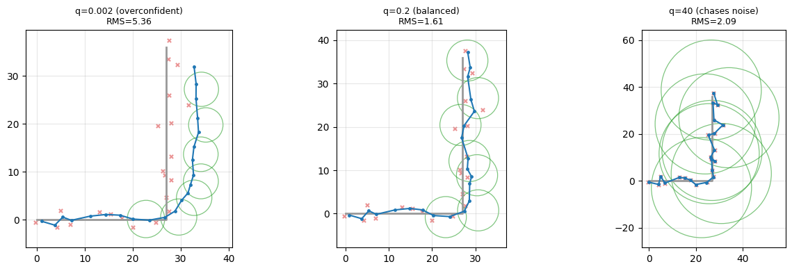
6c — Failure: mistuned noise (`q` too small vs. too large)

q encodes "how much can the object surprise me between frames?" Set it too small and the filter is overconfident: tight ellipses, sluggish to follow the maneuver, the estimate lags badly. Set it too large and the filter distrusts its own model, chases every noisy detection, and the estimate is jittery. Only the middle setting both follows the turn and stays smooth — the RMS error is U-shaped in q. Same L-path as above, now with noisier detections so both failure modes show.

g = torch.Generator().manual_seed(31)
meas_n = truth + 1.6 * torch.randn(T, 2, generator=g)   # noisier detections

fig, axes = plt.subplots(1, 3, figsize=(13, 4))
for ax, q, label in [(axes[0], 0.002, "q=0.002 (overconfident)"),
                     (axes[1], 0.2, "q=0.2 (balanced)"),
                     (axes[2], 40.0, "q=40 (chases noise)")]:
    proc = KalmanCentroid2D("centroid", q=q, r=2.5)
    rec = run_kalman(proc, torch.tensor([0., 0, 3, 0]),
                     torch.eye(4) * 2.0, list(meas_n), [True] * T)
    est = torch.stack([r["post_mean"][:2] for r in rec])
    rms = (est - truth).pow(2).sum(1).mean().sqrt()
    ax.plot(truth[:, 0], truth[:, 1], "-", color="0.6", lw=2)
    ax.scatter(meas_n[:, 0], meas_n[:, 1], marker="x", color="tab:red", s=14,
               alpha=0.5)
    ax.plot(est[:, 0], est[:, 1], "o-", color="tab:blue", ms=2.5)
    for k in range(8, T, 2):
        mu, S = predictive_xy(rec[k], proc.r)
        cov_ellipse(ax, mu, S, n_std=2.0, edgecolor="tab:green", lw=0.9,
                    alpha=0.6)
    ax.set_title(f"{label}\nRMS={rms:.2f}", fontsize=9)
    ax.set_aspect("equal"); ax.grid(alpha=0.3)
plt.tight_layout(); plt.show()

6d — Failure: crossing targets and ambiguous gates

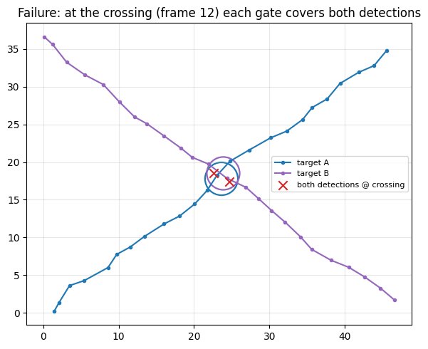
Motion prediction alone cannot keep two identities apart when their predictive distributions overlap. Two objects cross paths; near the crossing, each filter's 2σ ellipse contains both detections, so the association is a coin-flip — this is the classic point at which a pure-motion tracker swaps IDs. The lesson is structural: Kalman motion is necessary but not sufficient; an appearance cue (section 5) is what breaks the tie. The shaded frame marks the ambiguous window.

T = 24
t = torch.arange(T).float()
# Two targets crossing at the midpoint.
A = torch.stack([2.0 * t, 1.5 * t], dim=1)
B = torch.stack([2.0 * t, 36.0 - 1.5 * t], dim=1)
g = torch.Generator().manual_seed(27)
mA = A + 0.7 * torch.randn(T, 2, generator=g)
mB = B + 0.7 * torch.randn(T, 2, generator=g)

def track(meas, vy):
    proc = KalmanCentroid2D("centroid", q=0.05, r=0.5)
    m0 = torch.tensor([float(meas[0, 0]), float(meas[0, 1]), 2.0, vy])
    return proc, run_kalman(proc, m0, torch.eye(4) * 2.0, list(meas), [True] * T)

procA, recA = track(mA, 1.5)
procB, recB = track(mB, -1.5)

# Find the most ambiguous frame: ellipses closest / most overlapping.
kx = int(torch.argmin(torch.stack(
    [(recA[k]["prior_mean"][:2] - recB[k]["prior_mean"][:2]).norm()
     for k in range(T)])))

fig, ax = plt.subplots(figsize=(8, 5))
for rec_, proc_, col, name in [(recA, procA, "tab:blue", "target A"),
                               (recB, procB, "tab:purple", "target B")]:
    est = torch.stack([r["post_mean"][:2] for r in rec_])
    ax.plot(est[:, 0], est[:, 1], "o-", color=col, ms=3, label=name)
    mu, S = predictive_xy(rec_[kx], proc_.r)
    cov_ellipse(ax, mu, S, n_std=2.0, edgecolor=col, lw=1.6)
ax.scatter([float(mA[kx, 0]), float(mB[kx, 0])],
           [float(mA[kx, 1]), float(mB[kx, 1])],
           marker="x", color="tab:red", s=80, zorder=4,
           label="both detections @ crossing")
ax.set_title(f"Failure: at the crossing (frame {kx}) each gate covers both detections")
ax.legend(fontsize=8); ax.grid(alpha=0.3); ax.set_aspect("equal")
plt.tight_layout(); plt.show()

6e — Success: estimating a state you never measure

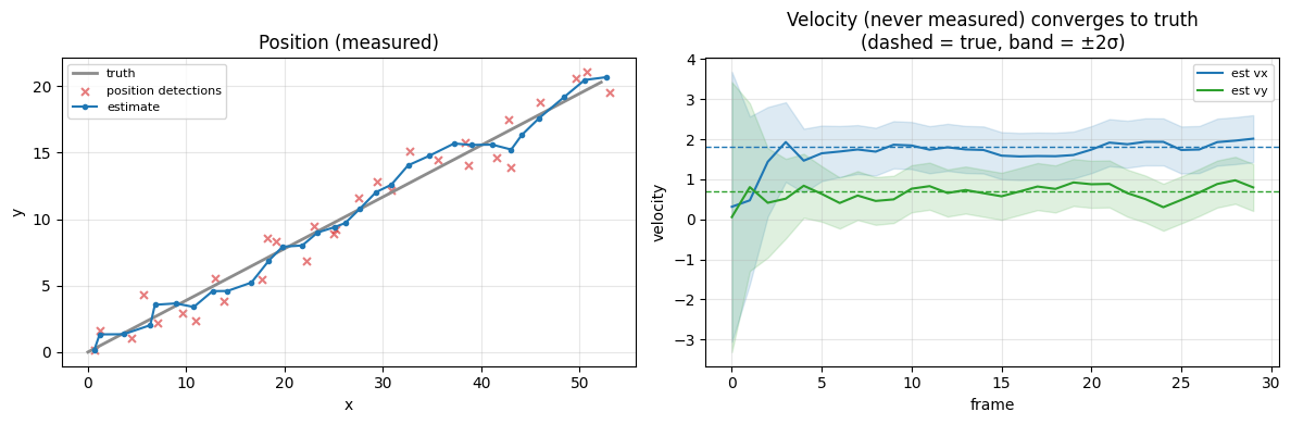
The detector reports only position, yet the filter needs velocity to predict. The Kalman filter infers it: velocity is an unobserved part of the state, and the correlations F induces between position and velocity let measurements of position update the velocity belief too. Below we deliberately initialise velocity at zero (wrong); within a handful of frames the estimated (vx, vy) lock onto the true values, and the ±2σ band — read straight off the covariance — shrinks as confidence grows. Nothing ever measured velocity directly.

T = 30
t = torch.arange(T).float()
true_v = torch.tensor([1.8, 0.7])
truth = t[:, None] * true_v                       # constant velocity
g = torch.Generator().manual_seed(33)
meas = truth + 1.2 * torch.randn(T, 2, generator=g)

proc = KalmanCentroid2D("centroid", q=0.02, r=1.44)
m0 = torch.tensor([0.0, 0.0, 0.0, 0.0])           # WRONG: zero velocity
rec = run_kalman(proc, m0, torch.eye(4) * 5.0, list(meas), [True] * T)

est = torch.stack([r["post_mean"] for r in rec])   # [x, y, vx, vy]
std = torch.stack([r["post_cov"].diagonal().clamp(min=0).sqrt() for r in rec])

fig, (axp, axv) = plt.subplots(1, 2, figsize=(12, 4))
axp.plot(truth[:, 0], truth[:, 1], "-", color="0.55", lw=2, label="truth")
axp.scatter(meas[:, 0], meas[:, 1], marker="x", color="tab:red", s=25,
            alpha=0.6, label="position detections")
axp.plot(est[:, 0], est[:, 1], "o-", color="tab:blue", ms=3, label="estimate")
axp.set_title("Position (measured)"); axp.legend(fontsize=8); axp.grid(alpha=0.3)
axp.set_xlabel("x"); axp.set_ylabel("y")

for j, name, col in [(2, "vx", "tab:blue"), (3, "vy", "tab:green")]:
    axv.plot(t, est[:, j], "-", color=col, label=f"est {name}")
    axv.fill_between(t, est[:, j] - 2 * std[:, j], est[:, j] + 2 * std[:, j],
                     color=col, alpha=0.15)
    axv.axhline(float(true_v[j - 2]), ls="--", color=col, lw=1)
axv.set_title("Velocity (never measured) converges to truth\n(dashed = true, band = ±2σ)")
axv.set_xlabel("frame"); axv.set_ylabel("velocity"); axv.legend(fontsize=8)
axv.grid(alpha=0.3)
plt.tight_layout(); plt.show()

6f — Failure, then fix: a clutter detection (outlier)

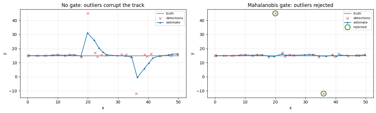
Kalman assumes Gaussian noise, so a single gross outlier — a false positive, a detection snapped to the wrong object — is wildly unlikely under the model, and the filter has no idea it should distrust it. Fused naively, one outlier yanks the estimate off the track for several frames (left). The standard defense is a gate: reject any detection whose Mahalanobis distance to the predictive distribution is too large (here χ² > 9.21, the 99% bound for 2 dof), treating it as a miss. The same two outliers are now rejected and the track stays clean (right). This is exactly why association in a real tracker runs through the predictive gate.

T = 26
t = torch.arange(T).float()
truth = torch.stack([2.0 * t, 15.0 + torch.zeros(T)], dim=1)
g = torch.Generator().manual_seed(35)
meas = truth + 0.8 * torch.randn(T, 2, generator=g)
meas[10] = torch.tensor([20.0, 45.0])             # clutter
meas[18] = torch.tensor([36.0, -12.0])            # clutter

def make_proc():
    return KalmanCentroid2D("centroid", q=0.05, r=0.7)
m0 = torch.tensor([0.0, 15.0, 2.0, 0.0])
rec_no = run_kalman(make_proc(), m0, torch.eye(4) * 2.0, list(meas), [True] * T)
rec_g = run_kalman(make_proc(), m0, torch.eye(4) * 2.0, list(meas), [True] * T,
                   gate_chi2=9.21)

fig, axes = plt.subplots(1, 2, figsize=(13, 4))
for ax, rec, title in [(axes[0], rec_no, "No gate: outliers corrupt the track"),
                       (axes[1], rec_g, "Mahalanobis gate: outliers rejected")]:
    est = torch.stack([r["post_mean"][:2] for r in rec])
    ax.plot(truth[:, 0], truth[:, 1], "-", color="0.6", lw=2, label="truth")
    ax.scatter(meas[:, 0], meas[:, 1], marker="x", color="tab:red", s=30,
               alpha=0.6, label="detections")
    ax.plot(est[:, 0], est[:, 1], "o-", color="tab:blue", ms=3, label="estimate")
    gated = [k for k, r in enumerate(rec) if r["gated"]]
    if gated:
        ax.scatter(meas[gated, 0], meas[gated, 1], s=160, facecolors="none",
                   edgecolors="tab:green", linewidths=2, label="rejected")
    ax.set_title(title); ax.legend(fontsize=8); ax.grid(alpha=0.3)
    ax.set_xlabel("x"); ax.set_ylabel("y")
plt.tight_layout(); plt.show()

6g — Failure: constant acceleration → systematic lag

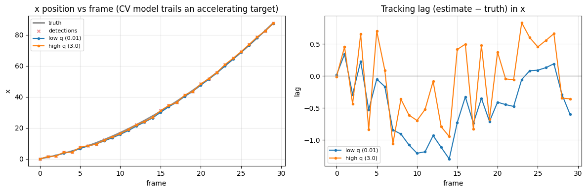
Section 6b broke the filter with a sharp turn. A smooth violation is sneakier: a target under constant acceleration. The constant-velocity model never predicts the speed-up, so its estimate trails the truth by a roughly constant lag that the update step can shrink but never erase — a persistent bias, not noise. Raising q lets the filter believe the velocity can change and cuts the lag, but the principled fix is a constant-acceleration model. The right panel shows the lag stays bounded-but-nonzero for low q.

T = 30
t = torch.arange(T).float()
accel = 0.14
x = 0.5 * accel * t ** 2 + 1.0 * t                # accelerating along x
truth = torch.stack([x, torch.zeros(T)], dim=1)
g = torch.Generator().manual_seed(37)
meas = truth + 0.5 * torch.randn(T, 2, generator=g)

runs = {}
for q, name in [(0.01, "low q (0.01)"), (3.0, "high q (3.0)")]:
    proc = KalmanCentroid2D("centroid", q=q, r=0.25)
    rec = run_kalman(proc, torch.tensor([0.0, 0.0, 1.0, 0.0]),
                     torch.eye(4) * 2.0, list(meas), [True] * T)
    runs[name] = torch.stack([r["post_mean"][:2] for r in rec])

fig, (axx, axl) = plt.subplots(1, 2, figsize=(12, 4))
axx.plot(t, truth[:, 0], "-", color="0.55", lw=2, label="truth")
axx.scatter(t, meas[:, 0], marker="x", color="tab:red", s=18, alpha=0.5,
            label="detections")
for name, est in runs.items():
    axx.plot(t, est[:, 0], "o-", ms=3, label=name)
axx.set_title("x position vs frame (CV model trails an accelerating target)")
axx.set_xlabel("frame"); axx.set_ylabel("x"); axx.legend(fontsize=8)
axx.grid(alpha=0.3)

for name, est in runs.items():
    axl.plot(t, (est[:, 0] - truth[:, 0]), "o-", ms=3, label=name)
axl.axhline(0, color="0.6", lw=1)
axl.set_title("Tracking lag (estimate − truth) in x")
axl.set_xlabel("frame"); axl.set_ylabel("lag"); axl.legend(fontsize=8)
axl.grid(alpha=0.3)
plt.tight_layout(); plt.show()

6h — Failure: a maneuver during a long occlusion

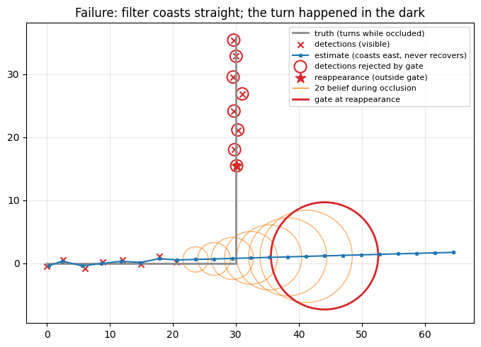
Two safe situations combine into a dangerous one. Coasting through an occlusion is fine if the motion stays constant (section 1); a maneuver is survivable if the object stays visible so the update can correct it (section 6b). But if the object turns while occluded, there is no measurement to catch the change: the filter coasts in a straight line, and when the object reappears the detection is nowhere near the prediction. Even with the occlusion-inflated gate, the true detection is rejected — the track is lost or, worse, steals a neighbour's detection.

# East for 11 frames, then north — but the turn falls inside the gap.
present = [True] * 8 + [False] * 7 + [True] * 8        # occluded 8..14
T = len(present)
truth = []
for k in range(T):
    if k <= 10:
        truth.append([3.0 * k, 0.0])                  # heading east
    else:
        truth.append([30.0, 3.0 * (k - 10)])          # turned north
truth = torch.tensor(truth)
g = torch.Generator().manual_seed(39)
meas = truth + 0.6 * torch.randn(T, 2, generator=g)

# A gated tracker: a reappearance outside the predictive gate is rejected.
proc = KalmanCentroid2D("centroid", q=0.05, r=0.4)
rec = run_kalman(proc, torch.tensor([0.0, 0.0, 3.0, 0.0]),
                 torch.eye(4) * 2.0, list(meas), present, gate_chi2=9.21)
est = torch.stack([r["post_mean"][:2] for r in rec])

fig, ax = plt.subplots(figsize=(8, 5))
ax.plot(truth[:, 0], truth[:, 1], "-", color="0.55", lw=2,
        label="truth (turns while occluded)")
seen = torch.tensor(present)
ax.scatter(meas[seen, 0], meas[seen, 1], marker="x", color="tab:red", s=35,
           label="detections (visible)")
ax.plot(est[:, 0], est[:, 1], "o-", color="tab:blue", ms=3,
        label="estimate (coasts east, never recovers)")
rej = [k for k, r in enumerate(rec) if r["gated"]]
if rej:
    ax.scatter(meas[rej, 0], meas[rej, 1], s=150, facecolors="none",
               edgecolors="tab:red", linewidths=1.5,
               label="detections rejected by gate")
# coasting belief through the gap
for k in range(T):
    if not present[k]:
        mu, S = predictive_xy(rec[k], proc.r)
        cov_ellipse(ax, mu, S, n_std=2.0, edgecolor="tab:orange", lw=1.0,
                    alpha=0.6)
kf = 15                                               # reappearance frame
mu, S = predictive_xy(rec[kf], proc.r)
cov_ellipse(ax, mu, S, n_std=2.0, edgecolor="tab:red", lw=2)
ax.scatter([float(meas[kf, 0])], [float(meas[kf, 1])], s=120, color="tab:red",
           marker="*", zorder=5, label="reappearance (outside gate)")
ax.plot([], [], color="tab:orange", lw=1.0, label="2σ belief during occlusion")
ax.plot([], [], color="tab:red", lw=2, label="gate at reappearance")
ax.set_title("Failure: filter coasts straight; the turn happened in the dark")
ax.legend(fontsize=8); ax.grid(alpha=0.3); ax.set_aspect("equal")
plt.tight_layout(); plt.show()

6i — Success: irregular frame rates (dt-aware prediction)

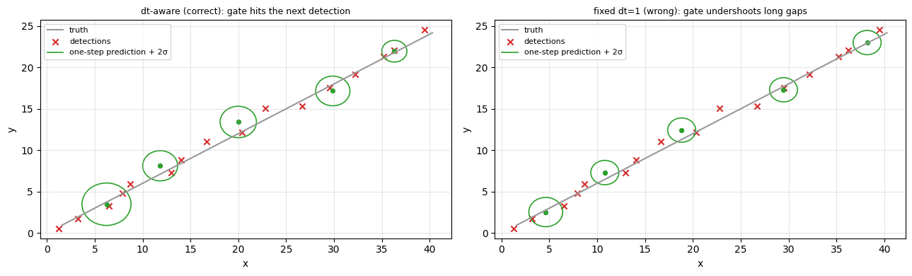
Real video is not metronomic: frames drop, sensors run at different rates, clips are sampled unevenly. unitrack's Kalman processes take the time step from ctx.delta, so F advances by the actual dt and Q injects q · dt of process noise — predictions and gates stay calibrated across uneven gaps. The left panel passes the true per-frame dt; the right wrongly assumes a fixed dt = 1. With the true dt the one-step predictions (green) land on the next detection; with a fixed dt they undershoot the long gaps and the gate sits behind the object — the kind of silent miscalibration that quietly loses tracks.

T = 16
g = torch.Generator().manual_seed(41)
dts = (0.4 + 1.6 * torch.rand(T, generator=g))        # irregular steps
times = torch.cumsum(dts, 0)
vel = torch.tensor([2.0, 1.2])
truth = times[:, None] * vel                          # CV in continuous time
meas = truth + 0.4 * torch.randn(T, 2, generator=g)

m0 = torch.tensor([float(meas[0, 0]), float(meas[0, 1]), 2.0, 1.2])
rec_ok = run_kalman(KalmanCentroid2D("centroid", q=0.05, r=0.16),
                    m0, torch.eye(4) * 1.0, list(meas), [True] * T,
                    dts=list(dts))
rec_bad = run_kalman(KalmanCentroid2D("centroid", q=0.05, r=0.16),
                     m0, torch.eye(4) * 1.0, list(meas), [True] * T,
                     dt=1.0)                            # ignores real dt

fig, axes = plt.subplots(1, 2, figsize=(13, 4))
for ax, rec, title in [(axes[0], rec_ok, "dt-aware (correct): gate hits the next detection"),
                       (axes[1], rec_bad, "fixed dt=1 (wrong): gate undershoots long gaps")]:
    ax.plot(truth[:, 0], truth[:, 1], "-", color="0.6", lw=1.5, label="truth")
    ax.scatter(meas[:, 0], meas[:, 1], marker="x", color="tab:red", s=35,
               label="detections")
    for k in range(2, T, 3):
        mu, S = predictive_xy(rec[k], 0.16)
        cov_ellipse(ax, mu, S, n_std=2.0, edgecolor="tab:green", lw=1.2)
        ax.scatter([float(mu[0])], [float(mu[1])], color="tab:green", s=18)
    ax.plot([], [], color="tab:green", lw=1.2, label="one-step prediction + 2σ")
    ax.set_title(title, fontsize=9); ax.legend(fontsize=8); ax.grid(alpha=0.3)
    ax.set_xlabel("x"); ax.set_ylabel("y")
plt.tight_layout(); plt.show()

Takeaways

Predict + update is the whole filter. Predict produces a distribution over the next measurement; update fuses a detection and shrinks it. The ellipses/ellipsoids in every plot are that predictive distribution — and they double as the association gate.
The state type only changes F, H, and the measurement. Points, boxes, mask centroids, 3-D clouds and appearance kernels are all the same recursion with different matrices — which is why unitrack exposes them as one Process + KalmanUpdate family.
It excels at denoising steady motion, coasting through short occlusions, inferring states it never measures (velocity from position alone, 6e), and staying calibrated under irregular frame rates via dt-aware F/Q (6i).
It breaks under maneuvers (model mismatch, 6b), constant acceleration (systematic lag, 6g), bad q/r tuning (6c), non-Gaussian clutter unless you gate (6f), turns hidden inside a long occlusion (6h), and identity ambiguity when predictive gates overlap (6d). Tuning fixes some; the rest need a better motion model, an outlier gate, or an appearance partner.
The predictive gate is the workhorse. Almost every failure above is detected by asking "is the detection inside the 2σ ellipse?" — the same Mahalanobis test that rejects clutter (6f), flags a maneuver (6b), and exposes a miscalibrated dt (6i).

In unitrack you rarely drive the filter by hand as we did here. Drop any of these processes into a Tracker via state_entries(...) and the predict/update loop, gating, and lifecycle are handled for you — see the tutorial notebooks (notebook 5 covers states and lifecycle end to end).

Embedding filters 6 — summary & benchmark

Tutorial notebooks