Notebook

Embedding filters 3 — von Mises-Fisher (directional)

ReID embeddings are compared by cosine similarity, so they really live on the unit sphere, not in flat space — a Euclidean Kalman filter is the wrong geometry. The von Mises-Fisher distribution is the sphere's Gaussian: a mean direction mu (unit) and a concentration kappa (certainty). Its mean direction has a conjugate vMF prior, so fusing an observation is an exact, closed-form update — the resultant of the concentration-weighted directions.

vmf_state_entries wires this up: match on mu with the ordinary Cosine cost, and read kappa as a live confidence.

import torch
import matplotlib.pyplot as plt

import unitrack
from unitrack.assignment import Associate, Jonker
from unitrack.costs import Cosine
from unitrack.data import Detections, FrameContext, TensorSpec
from unitrack.lifecycle import IncludeAll, NoLifecycle
from unitrack.pipeline import Pipe

torch.manual_seed(0)

D = 16          # embedding dimensionality (256+ in practice; 16 plots fast)
T = 44          # frames

def make_clip(noise=0.15, seed=0, switch=None):
    """
    A unit embedding that rotates slowly in the (e0, e1) plane plus
    per-frame noise in all D dims. Rotating in a known plane means
    projecting onto dims (0, 1) shows the true path as a circle arc.
    `switch` optionally rotates the plane mid-clip (an appearance change).
    """
    g = torch.Generator().manual_seed(seed)
    t = torch.arange(T).float()
    theta = 0.10 * t
    truth = torch.zeros(T, D)
    truth[:, 0] = torch.cos(theta)
    truth[:, 1] = torch.sin(theta)
    if switch is not None:
        # after `switch`, swap appearance into the (e2, e3) plane.
        truth[switch:, :] = 0.0
        truth[switch:, 2] = torch.cos(theta[switch:])
        truth[switch:, 3] = torch.sin(theta[switch:])
    obs = truth + noise * torch.randn(T, D, generator=g)
    obs = torch.nn.functional.normalize(obs, dim=-1)
    dets = [Detections(index=torch.tensor([0]), emb=obs[k:k + 1].clone(),
                       batch_size=[1]) for k in range(T)]
    return t, truth, obs, dets

def run(tracker, dets, fields=("emb",)):
    """Run a single-object clip through a real Tracker; collect snapshot fields."""
    ms = unitrack.MultiStream(tracker)
    rec = {f: [] for f in fields}
    for k, d in enumerate(dets):
        ctx = FrameContext.make(frame_idx=k, delta=1.0, fps=1.0, stream_key=0)
        res = ms.step(stream_key=0, detections=d, ctx=ctx)
        for f in fields:
            rec[f].append(getattr(res.snapshot, f)[0].clone())
    return {f: torch.stack(v) for f, v in rec.items()}

def cos_to_truth(est, truth):
    e = torch.nn.functional.normalize(est, dim=-1)
    u = torch.nn.functional.normalize(truth, dim=-1)
    return (e * u).sum(-1)

t, truth, obs, dets = make_clip()
print(f"clip: {T} frames, D={D}; raw-detection mean cosine-to-truth "
      f"= {cos_to_truth(obs, truth).mean():.3f}")

Output

clip: 44 frames, D=16; raw-detection mean cosine-to-truth = 0.855

from unitrack.states import vmf_state_entries

tracker = unitrack.Tracker(
    root=Pipe(cost=Cosine("emb"), assoc=Associate(Jonker(threshold=0.6))),
    states=vmf_state_entries("emb", dim=D, init_kappa=5.0,
                             kappa_obs=12.0, tau=8.0),
    lifecycle=NoLifecycle(), visibility=IncludeAll(),
)
rec = run(tracker, dets, fields=("emb", "emb_kappa"))

fig, (axp, axc) = plt.subplots(1, 2, figsize=(12, 4))
axp.plot(truth[:, 0], truth[:, 1], "-", color="0.55", lw=2, label="truth")
axp.scatter(obs[:, 0], obs[:, 1], marker="x", color="tab:red", s=22,
            alpha=0.5, label="noisy detections")
axp.plot(rec["emb"][:, 0], rec["emb"][:, 1], "o-", color="tab:blue",
         ms=3, label="filtered estimate")
axp.set_title("Embedding trajectory, projected to (dim 0, dim 1)")
axp.set_xlabel("dim 0"); axp.set_ylabel("dim 1")
axp.legend(fontsize=8); axp.grid(alpha=0.3); axp.set_aspect("equal")

axc.plot(t, cos_to_truth(obs, truth), color="tab:red", alpha=0.6,
         label="raw detections")
axc.plot(t, cos_to_truth(rec["emb"], truth), color="tab:blue",
         label="filtered")
axc.set_title("Cosine similarity to ground truth (higher = better)")
axc.set_xlabel("frame"); axc.set_ylabel("cosine"); axc.legend(fontsize=8)
axc.grid(alpha=0.3)

plt.tight_layout(); plt.show()
print(f"raw mean cos = {cos_to_truth(obs, truth).mean():.3f}   "
      f"filtered mean cos = {cos_to_truth(rec['emb'], truth).mean():.3f}")

Output

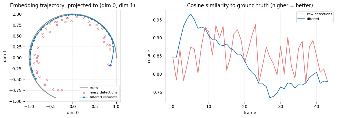
raw mean cos = 0.855   filtered mean cos = 0.832

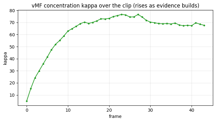
Concentration = confidence

The update sharpens the belief (kappa grows) as consistent detections accumulate; the predict step lets it decay, so a track that stops being seen becomes less certain of its appearance — a principled, geometry-aware confidence you can feed to a gate.

fig, ax = plt.subplots(figsize=(7, 4))
ax.plot(t, rec["emb_kappa"], "o-", color="tab:green", ms=3)
ax.set_title("vMF concentration kappa over the clip (rises as evidence builds)")
ax.set_xlabel("frame"); ax.set_ylabel("kappa")
ax.grid(alpha=0.3)
plt.tight_layout(); plt.show()
print(f"mu stays unit: max |‖mu‖ - 1| = "
      f"{(rec['emb'].norm(dim=-1) - 1).abs().max():.2e}")

Output

mu stays unit: max |‖mu‖ - 1| = 1.19e-07

Takeaway. vMF is the right filter for normalised embeddings: the estimate provably stays on the sphere and kappa is an honest directional confidence. It is the directional analogue of the Kalman filter in notebook 2.

Embedding filters 2 — Diagonal Kalman

Embedding filters 4 — Ensemble Kalman & information filters