Notebook

Embedding filters 6 — summary & benchmark

Seven recursive estimators for a tracker's appearance embedding, all behind the same State interface. This notebook puts them side-by-side on compute (FLOPs + wall-clock, and how they scale with the embedding dimension D), accuracy (on two complementary tasks), and effort (tuning / training), and ends with a fail/success cheat-sheet.

Method	one-line idea
EMA	constant-gain blend (steady-state scalar Kalman)
diagonal Kalman	random-walk Kalman, adaptive gain
vMF	recursive Bayes on the unit sphere
information filter	exact Kalman dual; additive fusion
EnKF	covariance via an ensemble (built for large `D`)
gallery	feature bank of the last `K` views
learned	MOTR-style module trained through the association

Methodology. Compute is measured on the state update in isolation (the matching cost is shared). Accuracy is measured on two tasks because no single number is fair to all: a denoising task (smooth a drifting embedding) and an association-under-fast-motion task (keep four rotating identities matched). Each method is set to a reasonable operating point — and finding that point is itself part of the "effort" comparison (vMF needs its decay tuned; the EnKF needs enough inflation or its ensemble collapses).

import time
import torch
import torch.nn as nn
import matplotlib.pyplot as plt

import unitrack
from unitrack.assignment import Associate, Jonker, sinkhorn_log_plan
from unitrack.costs import Cosine, GalleryCost
from unitrack.data import (
    Detections,
    FrameContext,
    MatchOutcome,
    TensorSpec,
    Tracklets,
)
from unitrack.lifecycle import IncludeAll, NoLifecycle
from unitrack.pipeline import Pipe
from unitrack.states import (
    EMAFuse,
    EMATrack,
    FromDetectionField,
    Identity,
    LearnedObservation,
    LearnedProcess,
    NoopObservation,
    NoopProcess,
    Replace,
    State,
    EyeInitializer,
    vmf_state_entries,
    gallery_state_entries,
)
from unitrack.states.kalman import (
    KalmanLinear,
    KalmanUpdate,
    enkf_state_entries,
    information_state_entries,
)

torch.manual_seed(0)


def _reserved(n):
    return dict(
        id=torch.arange(n),
        status=torch.full((n,), 1, dtype=torch.int8),
        hits=torch.ones(n, dtype=torch.int32),
        time_since_update=torch.zeros(n, dtype=torch.int32),
        age=torch.ones(n, dtype=torch.int32),
        frame_started=torch.zeros(n, dtype=torch.int32),
        frame_last_seen=torch.zeros(n, dtype=torch.int32),
    )


def spawn(states, n, dim):
    ds = Detections(index=torch.arange(n), emb=torch.randn(n, dim), batch_size=[n])
    user = {k: st.init(ds, FrameContext.make(0)) for k, st in states.items()}
    return Tracklets(**_reserved(n), **user, batch_size=[n]), ds


def match_n(n):
    p = torch.stack([torch.arange(n), torch.arange(n)], 1)
    return MatchOutcome(
        matched_pairs=p,
        tracklets_residual_index=torch.zeros(0, dtype=torch.int64),
        detections_residual_index=torch.zeros(0, dtype=torch.int64),
        per_match_cost=torch.zeros(n),
        batch_size=[],
    )


def step_update(states, cs, ds, m, ctx):
    out = cs
    for st in states.values():
        out = st.process(out, ctx)
    for st in states.values():
        out = st.observation(out, ds, m, ctx)
    return out


def time_us(fn, iters=40, warmup=5):
    for _ in range(warmup):
        fn()
    t0 = time.perf_counter()
    for _ in range(iters):
        fn()
    return (time.perf_counter() - t0) / iters * 1e6

# Method registry: a factory (states at dim D) + metadata, each at a
# reasonable operating point (see the per-method notebooks).
def st_ema(D):
    return {
        "emb": State(
            TensorSpec((D,), torch.float32),
            EMATrack("emb"),
            EMAFuse("emb", 0.8),
            FromDetectionField("emb"),
        )
    }


def st_kalman(D):
    e = torch.eye(D)
    return {
        "emb": State(
            TensorSpec((D,), torch.float32),
            KalmanLinear("emb", e, e, e * 0.02, e * 0.2),
            KalmanUpdate("emb", "emb_cov", e, e * 0.2),
            FromDetectionField("emb"),
        ),
        "emb_cov": State(
            TensorSpec((D, D), torch.float32),
            NoopProcess(),
            NoopObservation(),
            EyeInitializer(D, 1.0),
        ),
    }


def st_vmf(D):
    return vmf_state_entries("emb", dim=D, init_kappa=3.0, kappa_obs=5.0, tau=3.0)


def st_info(D):
    return information_state_entries("emb", dim=D, q=0.02, r=0.2)


def st_enkf(D):
    return enkf_state_entries(
        "emb", dim=D, ensemble_size=32, q=1.0, r=0.2, init_std=0.5
    )


def st_gallery(D):
    return gallery_state_entries("emb", dim=D, capacity=8)


def st_learned(D):
    prop = nn.Sequential(nn.Linear(D, 64), nn.Tanh(), nn.Linear(64, D))
    fuse = nn.Sequential(nn.Linear(2 * D, 64), nn.Tanh(), nn.Linear(64, D))
    nrm = torch.nn.functional.normalize
    return {
        "emb": State(
            TensorSpec((D,), torch.float32),
            LearnedProcess("emb", lambda x, dt: nrm(x + prop(x), dim=-1)),
            LearnedObservation(
                "emb",
                "emb",
                lambda tr, me: nrm(tr + fuse(torch.cat([tr, me], -1)), dim=-1),
            ),
            FromDetectionField("emb"),
        )
    }


METHODS = {
    "EMA": dict(make=st_ema, flops="2·N·D", effort=1),
    "diag-Kalman": dict(make=st_kalman, flops="~N·D³ (dense)", effort=2),
    "vMF": dict(make=st_vmf, flops="~4·N·D", effort=3),
    "info-filter": dict(make=st_info, flops="~N·D³", effort=3),
    "EnKF (E=32)": dict(make=st_enkf, flops="N·(E²D+E³)", effort=4),
    "gallery (K=8)": dict(make=st_gallery, flops="N·D  (+K·matching)", effort=2),
    "learned": dict(make=st_learned, flops="2·N·D·H  (+train)", effort=5),
}
print("methods:", list(METHODS))

Output

methods: ['EMA', 'diag-Kalman', 'vMF', 'info-filter', 'EnKF (E=32)', 'gallery (K=8)', 'learned']

1 — Compute: FLOPs and how they scale with `D`

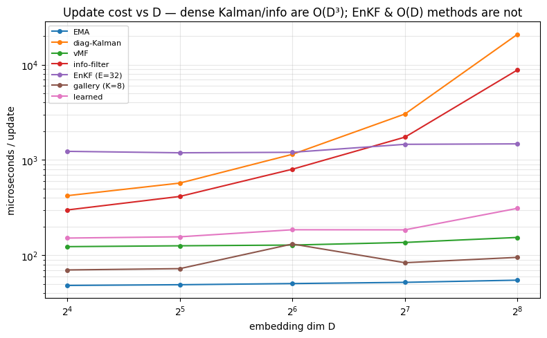
The dominant FLOPs of one state update (N tracks, D dims; E ensemble members, K gallery slots, H MLP width). The split is the whole point: the dense Gaussian filters are O(D³) per update (a D×D solve), which is fine at D=16 but ruinous at the D=256+ of a real ReID/DETR embedding. EMA, vMF and the learned MLP are O(D); the EnKF trades the D³ for E²D+E³, paying off once E ≪ D.

D_BENCH, N_BENCH = 256, 8
rows = []
with torch.no_grad():
    for name, meta in METHODS.items():
        st = meta["make"](D_BENCH)
        cs, ds = spawn(st, N_BENCH, D_BENCH)
        m = match_n(N_BENCH)
        ctx = FrameContext.make(1, delta=1.0)
        meta["us256"] = time_us(
            lambda st=st, cs=cs, ds=ds, m=m, ctx=ctx: step_update(st, cs, ds, m, ctx)
        )
        rows.append((name, meta["flops"], meta["us256"]))
print(f"state-update cost at D={D_BENCH}, N={N_BENCH}:")
for n, f, u in rows:
    print(f"  {n:14s} {f:22s} {u:9.1f} us")

fig, ax = plt.subplots(figsize=(9, 4))
names = [r[0] for r in rows]
us = [r[2] for r in rows]
ax.barh(names, us, color="tab:blue")
ax.set_xscale("log")
ax.set_xlabel("microseconds / update (log scale)")
ax.set_title(f"State-update wall-clock at D={D_BENCH} (N={N_BENCH} tracks)")
for i, u in enumerate(us):
    ax.text(u, i, f" {u:.0f}", va="center", fontsize=8)
ax.grid(alpha=0.3, axis="x")
plt.tight_layout()
plt.show()

Output

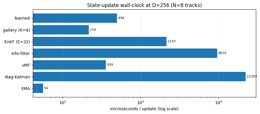
state-update cost at D=256, N=8:
  EMA            2·N·D                       56.0 us
  diag-Kalman    ~N·D³ (dense)            22393.3 us
  vMF            ~4·N·D                     359.5 us
  info-filter    ~N·D³                     9634.7 us
  EnKF (E=32)    N·(E²D+E³)                2147.4 us
  gallery (K=8)  N·D  (+K·matching)         215.8 us
  learned        2·N·D·H  (+train)          498.1 us

# Scaling with D: the O(D^3) filters curve up; the rest stay flat.
DIMS = [16, 32, 64, 128, 256]
curves = {name: [] for name in METHODS}
with torch.no_grad():
    for D in DIMS:
        for name, meta in METHODS.items():
            st = meta["make"](D)
            cs, ds = spawn(st, N_BENCH, D)
            m = match_n(N_BENCH)
            ctx = FrameContext.make(1, delta=1.0)
            curves[name].append(
                time_us(
                    lambda st=st, cs=cs, ds=ds, m=m, ctx=ctx: step_update(
                        st, cs, ds, m, ctx
                    ),
                    iters=25,
                )
            )
fig, ax = plt.subplots(figsize=(8, 5))
for name, ys in curves.items():
    ax.plot(DIMS, ys, "o-", ms=4, label=name)
ax.set_xscale("log", base=2)
ax.set_yscale("log")
ax.set_xlabel("embedding dim D")
ax.set_ylabel("microseconds / update")
ax.set_title(
    "Update cost vs D — dense Kalman/info are O(D³); EnKF & O(D) methods are not"
)
ax.legend(fontsize=8)
ax.grid(alpha=0.3, which="both")
plt.tight_layout()
plt.show()

Two honest caveats the benchmark exposes:

The shipped diagonal Kalman uses the generic dense KalmanLinear, so it is O(D³) here. A diagonal-specialised implementation would be O(D) — the math is cheap, the generic code is not.
The gallery's update is trivial (O(D) append); its real cost is in matching, where GalleryCost compares against K stored views — K× an ordinary cosine. We measure that separately:

D, N, M, K = 256, 8, 8, 8
gst = st_gallery(D)
gcs, _ = spawn(gst, N, D)
dets = Detections(index=torch.arange(M), emb=torch.randn(M, D), batch_size=[M])
ctx = FrameContext.make(0)
cos = Cosine("emb")
gcost = GalleryCost("emb_gallery", "emb_count", "emb")
t_cos = time_us(lambda: cos(gcs, dets, ctx))
t_gal = time_us(lambda: gcost(gcs, dets, ctx))
print(
    f"matching {N}x{M} at D={D}:  Cosine {t_cos:.1f} us   "
    f"GalleryCost(K={K}) {t_gal:.1f} us   ({t_gal / t_cos:.1f}x)"
)

Output

matching 8x8 at D=256:  Cosine 69.7 us   GalleryCost(K=8) 312.8 us   (4.5x)

2 — Accuracy on two complementary tasks

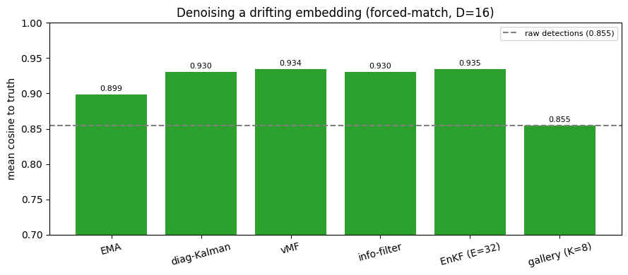
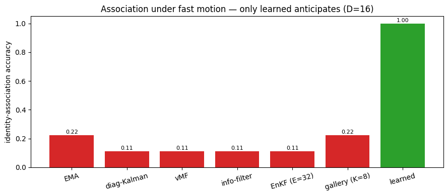
Denoising (smooth a drifting embedding): the genuine smoothers do well; the gallery sits at the raw level because it stores views rather than averaging them (it is memory, not a smoother), and learned is not built for this. Association under fast motion (four identities rotating ~54°/frame): every static filter lags into its neighbour and mis-associates; only the learned module, trained through the differentiable matcher, anticipates the motion.

D = 16


def dn_clip(T=44, noise=0.15, seed=0):
    g = torch.Generator().manual_seed(seed)
    t = torch.arange(T).float()
    th = 0.10 * t
    truth = torch.zeros(T, D)
    truth[:, 0] = torch.cos(th)
    truth[:, 1] = torch.sin(th)
    obs = torch.nn.functional.normalize(
        truth + noise * torch.randn(T, D, generator=g), dim=-1
    )
    return truth, obs


def denoise_cos(states):
    """Forced-match single-track driver: isolates filter quality from matching."""
    truth, obs = dn_clip()
    d0 = Detections(index=torch.tensor([0]), emb=obs[0:1].clone(), batch_size=[1])
    cs = Tracklets(
        **_reserved(1),
        **{k: st.init(d0, FrameContext.make(0)) for k, st in states.items()},
        batch_size=[1],
    )
    m = match_n(1)
    coss = []
    for k in range(1, len(obs)):
        ctx = FrameContext.make(k, delta=1.0)
        for st in states.values():
            cs = st.process(cs, ctx)
        ds = Detections(
            index=torch.tensor([0]), emb=obs[k : k + 1].clone(), batch_size=[1]
        )
        for st in states.values():
            cs = st.observation(cs, ds, m, ctx)
        coss.append((torch.nn.functional.normalize(cs.emb[0], dim=0) @ truth[k]).item())
    return sum(coss) / len(coss)


truth, obs = dn_clip()
raw = (torch.nn.functional.normalize(obs, dim=-1) * truth).sum(-1).mean().item()
denoise = {}
with torch.no_grad():
    for name in [
        "EMA",
        "diag-Kalman",
        "vMF",
        "info-filter",
        "EnKF (E=32)",
        "gallery (K=8)",
    ]:
        denoise[name] = denoise_cos(METHODS[name]["make"](D))
METHODS_denoise = denoise
fig, ax = plt.subplots(figsize=(9, 4))
names = list(denoise)
vals = [denoise[n] for n in names]
ax.bar(names, vals, color="tab:green")
ax.axhline(raw, ls="--", color="0.5", label=f"raw detections ({raw:.3f})")
ax.set_ylim(0.7, 1.0)
ax.set_ylabel("mean cosine to truth")
ax.set_title("Denoising a drifting embedding (forced-match, D=16)")
ax.legend(fontsize=8)
plt.xticks(rotation=15)
for i, v in enumerate(vals):
    ax.text(i, v + 0.005, f"{v:.3f}", ha="center", fontsize=8)
plt.tight_layout()
plt.show()

# Association task: rotate fast; learned anticipates, statics lag.
N, RT, OM, NZ = 4, 10, 0.95, 0.10


def rot_clip(seed, shuffle=True):
    g = torch.Generator().manual_seed(seed)
    ph = torch.arange(N).float() * (2 * torch.pi / N)
    frames, gts = [], []
    for k in range(RT):
        a = ph + OM * k
        e = torch.zeros(N, D)
        e[:, 0] = torch.cos(a)
        e[:, 1] = torch.sin(a)
        e = torch.nn.functional.normalize(
            e + NZ * torch.randn(N, D, generator=g), dim=-1
        )
        order = torch.randperm(N, generator=g) if shuffle else torch.arange(N)
        frames.append(e[order])
        gt = torch.empty(N, dtype=torch.long)
        gt[order] = torch.arange(N)
        gts.append(gt)
    return frames, gts


def assoc_acc(states):
    tr = unitrack.Tracker(
        root=Pipe(cost=Cosine("emb"), assoc=Associate(Jonker(threshold=0.95))),
        states=states,
        lifecycle=NoLifecycle(),
        visibility=IncludeAll(),
    )
    ms = unitrack.MultiStream(tr)
    frames, _ = rot_clip(99, shuffle=False)
    c = t = 0
    for k in range(RT):
        d = Detections(index=torch.arange(N), emb=frames[k].clone(), batch_size=[N])
        res = ms.step(
            stream_key=0,
            detections=d,
            ctx=FrameContext.make(k, delta=1.0, stream_key=0),
        )
        if k > 0:
            p = res.match.matched_pairs
            c += int((p[:, 0] == p[:, 1]).sum())
            t += p.shape[0]
    return c / max(t, 1)


# Train the learned propagator/fuser through the soft association (MOTR-style).
def cosdist(a, b):
    a = torch.nn.functional.normalize(a, dim=-1)
    b = torch.nn.functional.normalize(b, dim=-1)
    return 1.0 - a @ b.T


prop = nn.Sequential(nn.Linear(D, 64), nn.Tanh(), nn.Linear(64, D))
fuse = nn.Sequential(nn.Linear(2 * D, 64), nn.Tanh(), nn.Linear(64, D))
nrm = torch.nn.functional.normalize
pf = lambda x: nrm(x + prop(x), dim=-1)
ff = lambda tr, me: nrm(tr + fuse(torch.cat([tr, me], -1)), dim=-1)
opt = torch.optim.Adam(list(prop.parameters()) + list(fuse.parameters()), lr=3e-3)
for epoch in range(150):
    frames, gts = rot_clip(epoch)
    track = frames[0][gts[0]].clone()
    loss = 0.0
    for k in range(1, RT):
        pred = pf(track)
        logP = sinkhorn_log_plan(cosdist(pred, frames[k]), epsilon=0.05, num_iter=50)
        loss = loss - logP[torch.arange(N), gts[k]].mean()
        track = ff(pred, frames[k][gts[k]])
    opt.zero_grad()
    (loss / (RT - 1)).backward()
    opt.step()

learned_states = {
    "emb": State(
        TensorSpec((D,), torch.float32),
        LearnedProcess("emb", lambda x, dt: pf(x)),
        LearnedObservation("emb", "emb", ff),
        FromDetectionField("emb"),
    )
}

assoc = {}
with torch.no_grad():
    for name in [
        "EMA",
        "diag-Kalman",
        "vMF",
        "info-filter",
        "EnKF (E=32)",
        "gallery (K=8)",
    ]:
        assoc[name] = assoc_acc(METHODS[name]["make"](D))
    assoc["learned"] = assoc_acc(learned_states)
fig, ax = plt.subplots(figsize=(9, 4))
names = list(assoc)
vals = [assoc[n] for n in names]
cols = ["tab:red" if v < 0.5 else "tab:green" for v in vals]
ax.bar(names, vals, color=cols)
ax.set_ylim(0, 1.05)
ax.set_ylabel("identity-association accuracy")
ax.set_title("Association under fast motion — only learned anticipates (D=16)")
for i, v in enumerate(vals):
    ax.text(i, v + 0.01, f"{v:.2f}", ha="center", fontsize=8)
plt.xticks(rotation=15)
plt.tight_layout()
plt.show()

# ---- the side-by-side table ----
FAILSUCCESS = {
    "EMA": ("cheap default smoothing", "no uncertainty; reactive"),
    "diag-Kalman": ("adaptive uncertainty, small D", "dense O(D³) at large D"),
    "vMF": ("cosine/normalised embeddings", "needs decay tuning"),
    "info-filter": ("exact posterior; fuse cues", "O(D³); large D"),
    "EnKF (E=32)": ("full covariance at large D", "collapses w/o inflation"),
    "gallery (K=8)": ("appearance change / re-ID", "no smoothing; K× match"),
    "learned": ("anticipate complex motion", "needs training data"),
}
order = [
    "EMA",
    "diag-Kalman",
    "vMF",
    "info-filter",
    "EnKF (E=32)",
    "gallery (K=8)",
    "learned",
]
header = [
    "method",
    "FLOPs/update",
    "us@D256",
    "denoise",
    "assoc",
    "effort",
    "best for",
    "fails at",
]
cells = []
for n in order:
    cells.append(
        [
            n,
            METHODS[n]["flops"],
            f"{METHODS[n]['us256']:.0f}",
            f"{METHODS_denoise.get(n, float('nan')):.3f}"
            if n in METHODS_denoise
            else "—",
            f"{assoc.get(n, float('nan')):.2f}" if n in assoc else "—",
            "★" * METHODS[n]["effort"],
            FAILSUCCESS[n][0],
            FAILSUCCESS[n][1],
        ]
    )
fig, ax = plt.subplots(figsize=(16, 3.2))
ax.axis("off")
tbl = ax.table(
    cellText=cells,
    colLabels=header,
    loc="center",
    cellLoc="left",
    colWidths=[0.085, 0.13, 0.06, 0.06, 0.05, 0.07, 0.21, 0.21],
)
tbl.auto_set_font_size(False)
tbl.set_fontsize(8.5)
tbl.scale(1, 1.6)
for j in range(len(header)):
    tbl[0, j].set_facecolor("#dddddd")
    tbl[0, j].set_text_props(weight="bold")
ax.set_title("Embedding filters, side by side", fontsize=11, pad=12)
plt.tight_layout()
plt.show()

How to choose

Default to EMA. Cheapest, robust, one knob. Reach further only when it isn't enough.
Want calibrated uncertainty (for gating) and D is small → diagonal Kalman or the information filter (exact, and the IF fuses many cues by addition).
Embeddings are cosine-normalised and you want a confidence → vMF (just tune the decay to the drift rate).
D is large and you still want covariance → EnKF (give it enough inflation), the only O(D)-friendly full-covariance option.
Appearance changes / re-ID gaps → a gallery; it does not smooth, it remembers.
Motion is complex and you have data → a learned module, trained through the association — the only method that anticipates rather than reacts, at the cost of a training pipeline.

No method dominates: the dense filters denoise best but don't scale; the EnKF scales but must be inflated; the gallery and learned modules win tasks the smoothers structurally cannot. The shared State interface means you can swap among them — or compose them — without touching the rest of the tracker.

Embedding filters 5 — Memory bank & learned propagation

Kalman filters for motion prediction in tracking

Embedding filters 6 — summary & benchmark

1 — Compute: FLOPs and how they scale with D

2 — Accuracy on two complementary tasks

How to choose

1 — Compute: FLOPs and how they scale with `D`